Restricted Boltzmann Machines (RBM) are building blocks for certain type of neural networks which were invented by G.E.Hinton.
In a paper published in Science – Hinton describing how to use neural networks to reduce dimensionality of data using an autoencoder. Below is a sketch of a standard autoencoder where data is inserted from layer X on the left, code is for a data is presented in layer Z. The training of the network is done by adding a decoder network from the code layer on and calculate the error by the difference of the encoding at layer X’ to the original data in layer X then using back propagation to update the network weights.

One of the challenges of training deep autoencoder is that unless the network’s weights are initialize close to their optimum value – the training will fail and the encoder will not work. Hinton suggested a pre-train phase where every two layers up to the encoder layer are trained in separation from the other layers in that group. Once the first two layers are pre-trained than we move to the two layers where the last layer of the previous step becomes the first layer of the next pair. The graph below shows that a a network with 7 layers training is failing compared to a a network that was pre-trained.

RBM is a two layer network with the following constraints
- the layer on the left is called the visible layer and the one on the right is called the hidden layer
- symmetrical connections
- no connections between nodes within the same layer
- There are bias weights for both visible and hidden units

The pre-train is compose from the following steps (taken from wikipedia):

Comments on the pre-train procedure:
- ‘v’ is the visible vector, ‘h’ is the hidden later vector, ‘a’ is the bias vector of the visible layer and ‘b’ is the bias vector of the hidden layer.
- in step 1 – the hidden layer contains only 1 or 0 value. it is calculated in a stochastic process by generating a random number in the range (0,1) and if the value if h_i is greater than this random value h_i=1 otherwise h_i=0, same goes for step3.
- outer product is the matrix that is generated from multiplying the column vector v and the row vector h.
- epsilon is the learning rate
Each two layers of the encoder are pre-trained using the training data several times (this is also called epochs). When completing the pre-train of 2 layers then the hidden layer becomes the visible layer of the next pair of the encoder and it is pre-trained together with the next layer of the encoder in a greedy way.
When all layers up to the code layer are pre- trained then unrolling of the layer is done which means all matrix transpose are taken as weights to the encoder network. This described in the following sketch:

Now, the fine tune phase starts which is the standard autoencoder unsupervised learning via back propagation algorithm.
We are ready to encode! we will use the neural net from bottom layer up to the coding layer and pass through it our data for encoding.
Here are some results of encoding and then decoding using RBM which are compared to PCA algorithms, taken from Hinton’s paper:
Figure A
- Architecture: (28X28)-400-200-100-50-25-6
- Training: 20,000 images
- Testing: 10,000 new images.

Figure B
- Architecture: 784-1000-500-250-30.
- Training: 60,000 images
- Testing: 10,000 new images.

Figure C

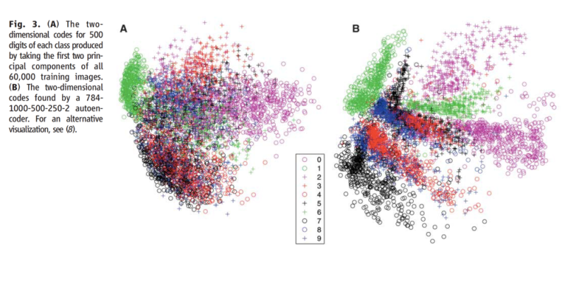
Figure showing visual clustering of RBM compared to PCA: